More than a year ago, I published a first post dedicated to the geolocation of a commercial flight from a photo taken in the plane and based on various research and open source tools. However, other tools exist and are, in my opinion, not enough covered in media. So I thought it would be interesting to write a few lines about them. And then, once again, like a running gag in our discussion groups, a photo also taken from a plane was sent to us. It turns out that this is a perfect case to introduce these tools.
Geolocation of a flight from a photo? Let’s go for episode 2!
Foreword
If you land on this post from an external source, I strongly advise you to start by reading my first post on the subject, available here.
In this second chapter, we will first solve this case through the “classic” method through the analysis and flight tracking tools. Then in a second time, and this is the main goal of this post, I would like to introduce a relatively powerful and maybe less known tool.
Context and first elements
In the same way as the first case solved on this blog, this story starts with the following photo, received on 10/29/2021 at 11:58 am, wondering who could tell where this person planned to spend his weekend.
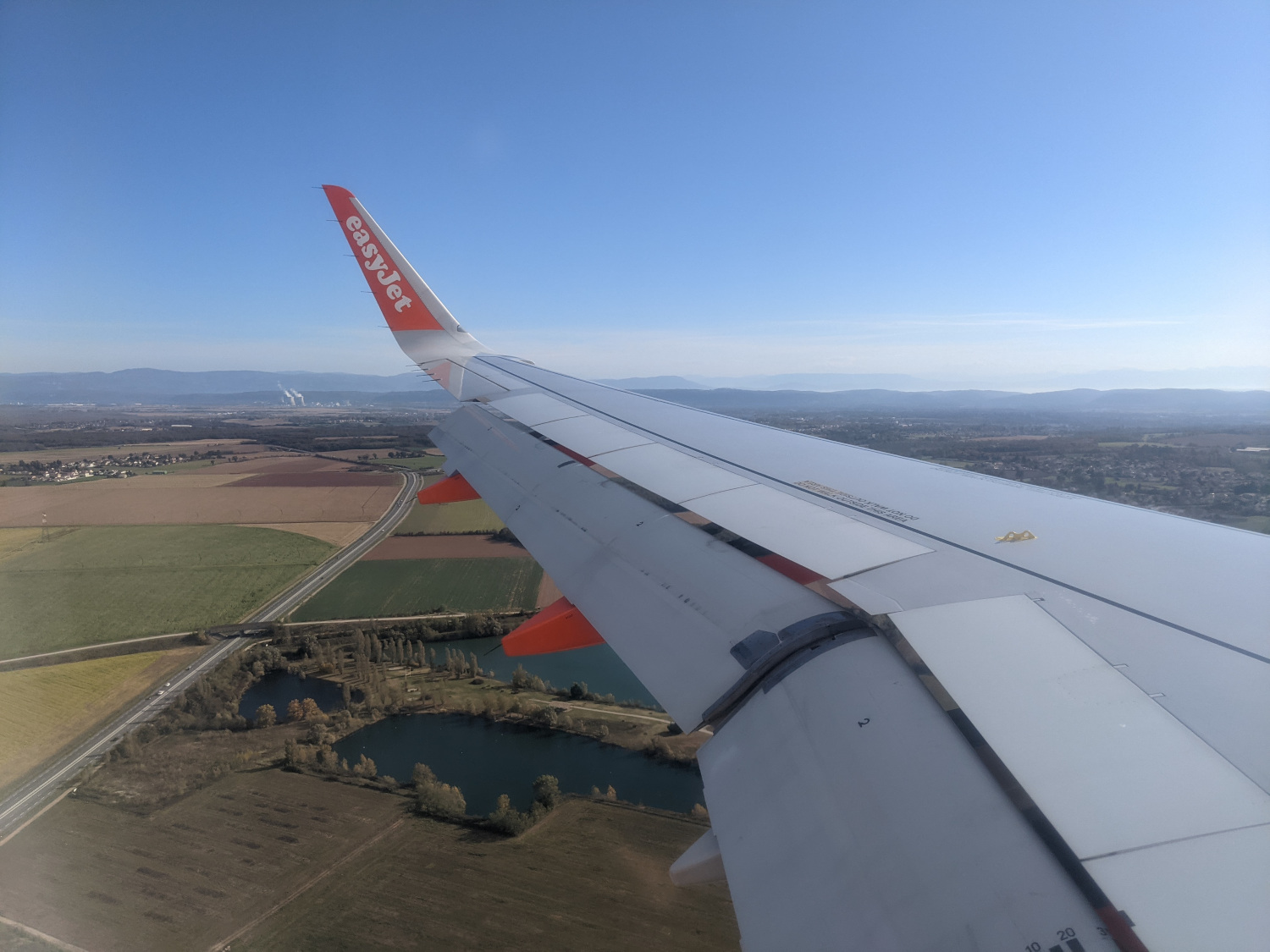
The file name is “PXL_20211029_095541933.jpg”. This time, no timestamp ! However, we can validate the date of the photo shot, which is indeed the 10/29/2021. It is also possible to verify this information through the picture metadata.
Indeed, by default, when uploading a photo on social platforms, the metadata are removed to clean up the files and save space. However, through Telegram (because this is where we got the image), it is possible to send an image as a raw file, without compression and thus keeping metadata.
$ exiftool PXL_20211029_095541933.jpg

[...]
Aperture                        : 1.7
Image Size                      : 4032x3024
Megapixels                      : 12.2
Scale Factor To 35 mm Equivalent: 6.2
Shutter Speed                   : 1/3906
Create Date                     : 2021:10:29 11:55:41.933+02:00
Date/Time Original              : 2021:10:29 11:55:41.933+02:00
Modify Date                     : 2021:10:29 11:55:41.933+02:00
Thumbnail Image                 : (Binary data 14521 bytes, use -b option to extract)
Circle Of Confusion             : 0.005 mm
Depth Of Field                  : inf (1.54 m - inf)
Field Of View                   : 67.4 deg
Focal Length                    : 4.4 mm (35 mm equivalent: 27.0 mm)
Hyperfocal Distance             : 2.28 m
Light Value                     : 14.2
Thanks to this, we know, among other things, that the photo was taken at 11:55 on 29/10/2021.
Good. Second step, the remarkable elements of the photo and what we can learn from them. Looks like a deja vu … Don’t you think so?
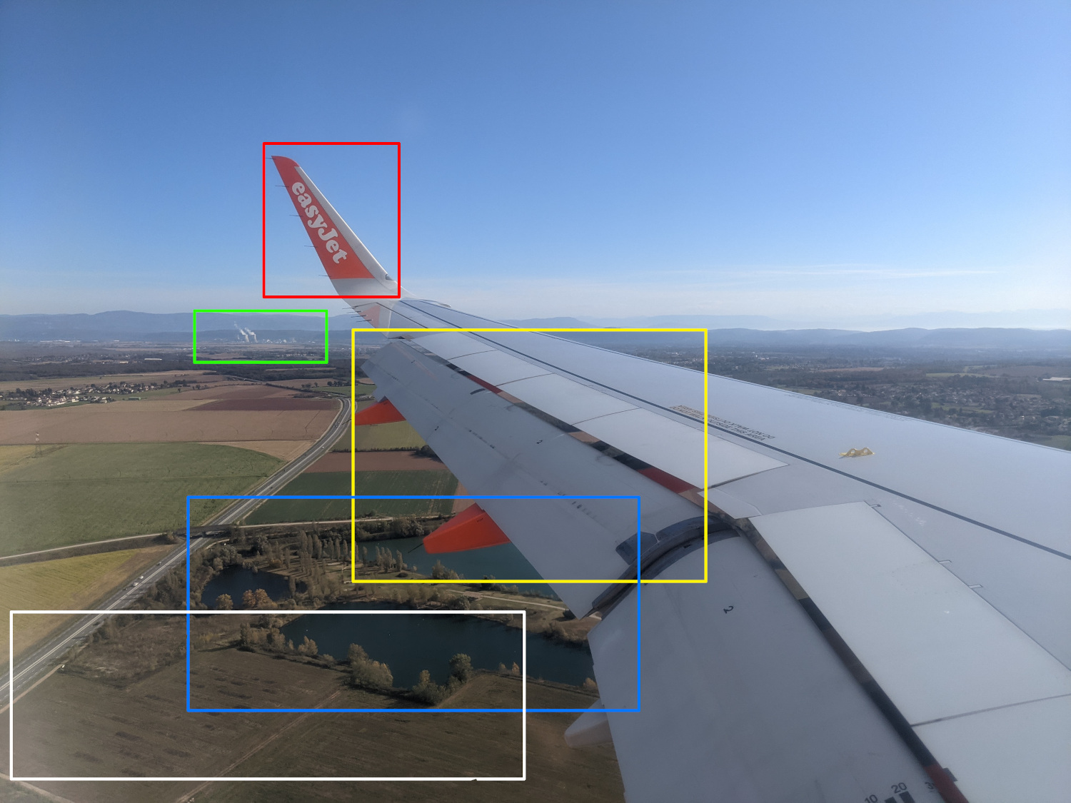
- White: The first thing to consider here is the altitude! Indeed, even if it seems obvious, it is probably the most important information. Indeed, the altitude being relatively low, it shows that the picture was taken just after the takeoff, or just before landing ;
- Red : Rather simple, the plane’s winglet gives us the airline (Easyjet) as well as an indication on the model of the aircraft ;
- Yellow: The wing flaps are deployed, which confirms the landing or takeoff ;
- Blue: A water source. Or rather three different water source. We will see it later, but this is typically the kind of remarkable geographical point we need ;
- Green: In the background, we can see an industrial site with two large “chimneys”, which looks very much like a nuclear power plant ;
- We could also note other interesting elements, such as a medium-sized road with 4 lanes, a bridge, or reliefs in the background.
Now, two methods, each using some elements of the image.
Method 1 : Classic, solving by flights analysis
If you have read my first post on this topic, this will looks familiar. Indeed, knowing the approximate time of the flight, and more precisely the landing time thanks to the low altitude of the aircraft as well as the company operating the flight, the identification can be done quite easily by means of various flight tracking and analysis tools.
I have mentioned this before, but the following tools allow free access to flight histories in a time-limited manner. Access to older data is also possible, but these are usually paid services.
Right. Knowing the date of the flight and having an idea of a range (the aircraft should be flying at 11:55), let’s start by looking at the flights operated by EasyJet on 10/29/2021. The Airportia tool (link) allows (among others) this type of search. Small precision, the person being French, we will focus on flights from cities located in France. Also note that the times displayed are in UTC format. In our case, it is therefore necessary to add 2 hours.
Based on these criteria, two flights match. However, given the image and the altitude, we can include flights that theoretically landed a few minutes before the time of the photo (potential delays, etc). In the end, 4 flights can be matched.
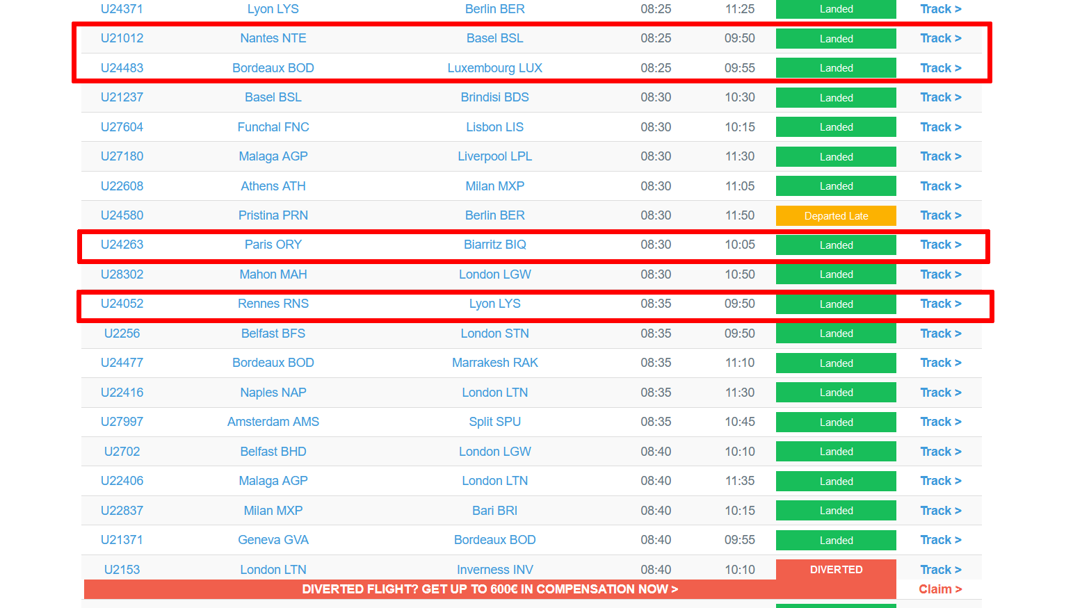
Four flights to analyze, it is quite little! Airportia also allows to have more precise details on a flight and in particular the real times of departure and arrival! Thus, it is possible to see the possible delays. Considering the altitude and the time of the photo, the flight U24263 (Paris-Biarritz) can be excluded since it landed about 10 minutes after the photo was taken, which is late compared to the position of the aircraft on this photo.
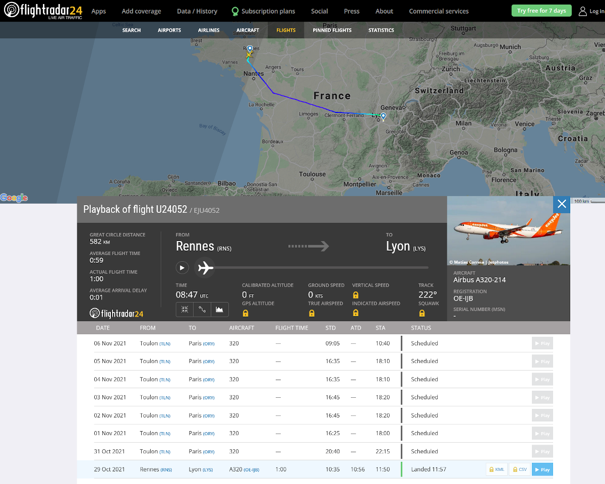
Other flights can match. However, flight U24052 (Rennes-Lyon) pulls attention thanks to a particular detail. Indeed, the information on this flight reveals that the flight of the day was delayed and that consequently, the landing took place at 11:57 am!
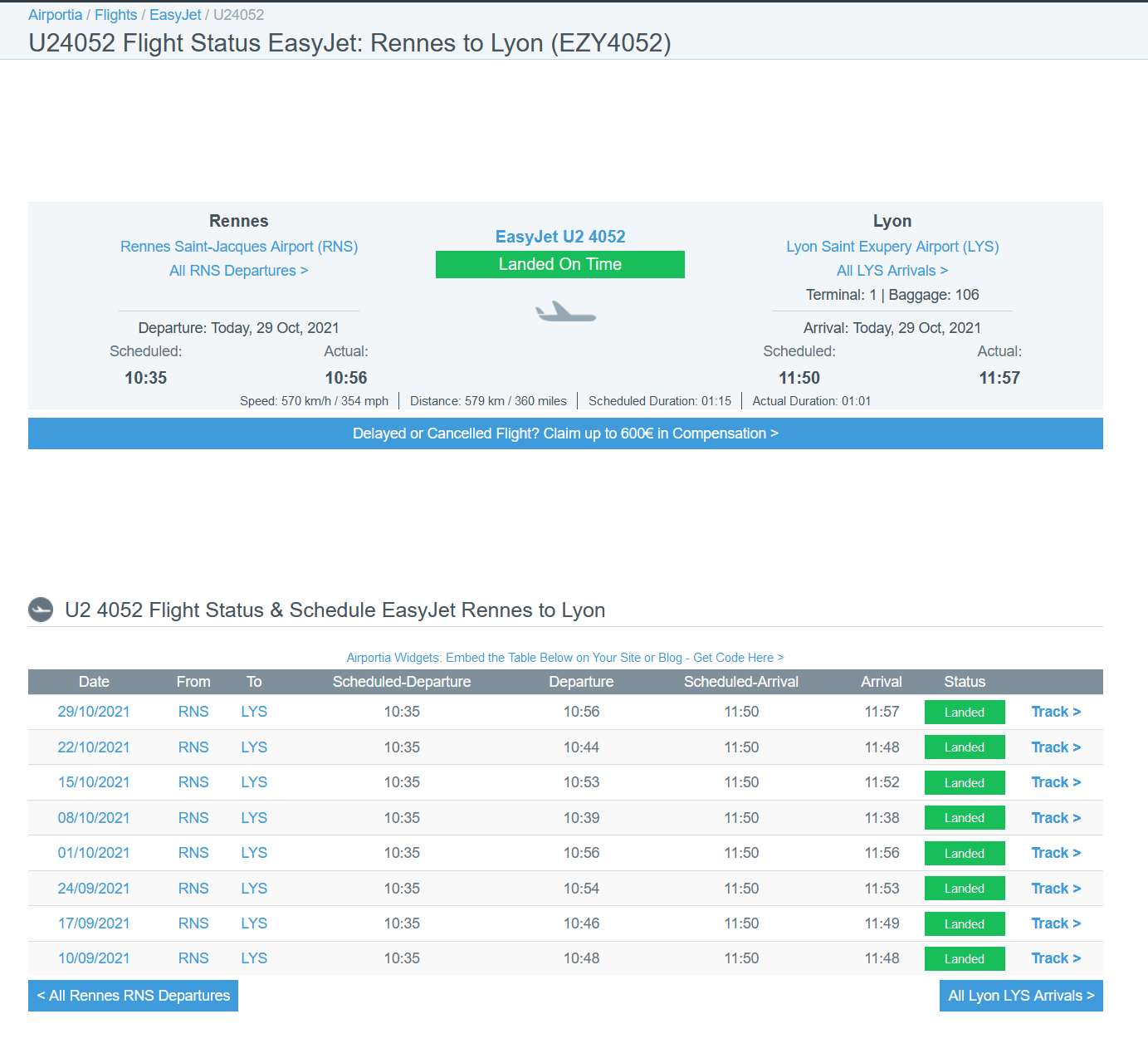
This flight seems to be a good candidate. Now, the FlightRadar24 tool (tool), also introduced in the first flight analysis post, was used. A great feature is the possibility to “replay” a flight once it has landed. This allows to know the route taken by the aircraft, minute by minute, and to have precise information such as the speed or the altitude at a given time. Thus, by searching for the target flight, it is possible to replay it.
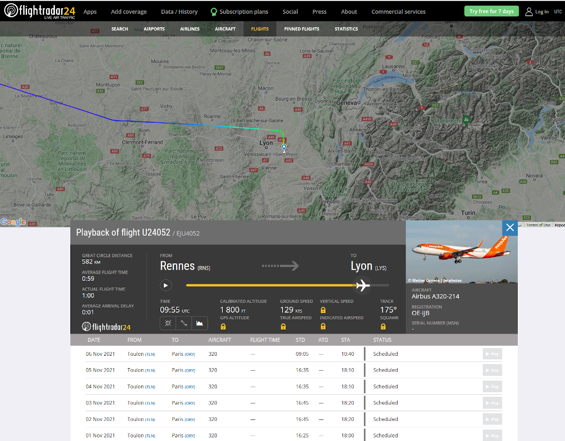
We position ourselves at the time of the photo shot, 11:55 (remember, 9:55 on the website because we are in UTC format) and we can see the position and orientation of the aircraft, as well as its altitude of 1800 feet. As I don’t know much about these scales, Google tells me that it corresponds to about 550 meters.
Good. We now know where this plane was at 11:55. Now we just have to look at the geographical environment near this position to say whether it is this flight or not. If it is not, then the analysis process can be repeated for the other identified flights.
By zooming in on the FlightRadar map, you can see the exact position with a “Google Maps” like map, also showing roads, railroads, water points… Did you say water point?
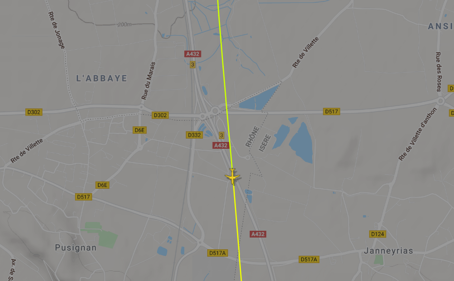
The image shows indeed several water points close to the position of the aircraft, on its left, which corresponds to our research. Moreover, we identified a particular linked feature. Indeed, the original image shows at least 3 water points with a shape rather close to those represented on the map.
Having the exact position of the aircraft as well as the potential water sources, we can now try to find more precise images of the area to see if it matches. The excellent Google Earth Pro is perfect for this purpose. We go to the indicated position of the device and after a slight orientation, we obtain the following image.
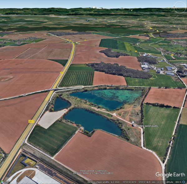
The water points, the road, the bridge, and even the industrial site in the background, everything is there! This confirms the airport of arrival as well as the supposed flight. We can therefore affirm that this person left Rennes in order to spend his weekend in Lyon’s region.
Ok… But now let’s suppose that we arrive a few days later and that we don’t want to pay to have access to the older flight data, can we still answer this question from the available elements?
Method 2 : Let me introduce… Overpass Turbo !
Now we come to the main part of this post ! As mentioned in the introduction, the idea is to quickly present a tool that is particularly useful in the analysis of geographic data and especially when it comes to geolocating elements.
In short, Overpass Turbo (link) is a tool for extracting and exploring data from the OpenStreetMap network. It allows to build queries, executed through the Overpass API and retrieve data on an interactive map.
In order to bring a quick definition (thanks Wikipedia), OpenStreetMap (OSM) is a collaborative online mapping project that aims to build a free geographic database of the world using GPS and other free data. Basically, each person can fill in real world elements on this map, following a few identification rules, which creates a great database, as you will see. By the way, OpenFacto made a great post about this topic 2 years ago, which I invite you to read as well.
Before we get into the nitty-gritty of the subject, here are a few things that are necessary to understand. Without going into details, the objects listed in OSM and searchable through Overpass Turbo can be of three different types:
- A node: These are the basic elements of the OSM system. Nodes consist of a latitude and a longitude. Basically, a point on the map ;
- A way: A way is an interconnection between two or more nodes that characterizes a line such as a street, or similar ;
- A relation : A relationship object is a collection of objects.
Thus, any feature registered with Open Street Map is categorized by at least one of these properties (more information here)
Moreover, each object is also associated with different properties (“features” and “tags”) that allow to define it, but also to search it. This categorization works in the form of keys/values. For example, a road will have the key highway as well as a value to define its importance. Thus, a highway will be characterized by the couple highway=motorway. On the other hand, a much less important road, connecting for example two villages, will be represented as highway=secondary.
Finally, it is also possible to add additional elements to filter the results, called “tags”. There is an astronomical amount of tags, specific to each type of object in OSM. If we take the example of roads, it is for example possible to use the tags lanes= or maxspeed.
The OpenStreetMap wiki references all the existing elements, as well as the tags that can be associated with them. It’s a real gold mine, absolutely essential to target correctly the searches: Map Features.
Good! Now we have all the basic theory to build an Overpass Turbo query. But what does an Overpass query look like?
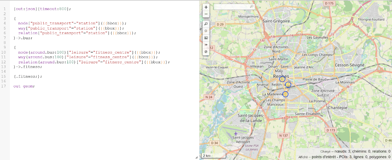
To illustrate this, here’s a simple example. Let’s say I regularly take the bus in Rennes (France) and I’m looking for a gym. However, lazy as I am, I would like this gym to be located relatively close to a bus stop. Well, in “Overpass” language, it looks like this:
[out:json][timeout:800];


(
  node["public_transport"="station"]({{bbox}});
  way["public_transport"="station"]({{bbox}});
  relation["public_transport"="station"]({{bbox}});
)->.bus;

(
  node(around.bus:100)["leisure"="fitness_centre"]({{bbox}});
  way(around.bus:100)["leisure"="fitness_centre"]({{bbox}});
  relation(around.bus:100)["leisure"="fitness_centre"]({{bbox}});
)->.fitness;

(.fitness;);

out geom;
Indeed, it is not very user-friendly. Nevertheless, once you understand the basic notions, you will see that you will find your way around. Some explanations:
- The instruction
[out:json][timeout:800];allows you to define the maximum search time before the search expires ; - The first block consists in searching all the nodes, paths and relations corresponding to bus stops. These can be referenced with the keys
public_transportand valuesstation(But not only! Other possible names are indicated on the OSM wiki). The result of this search is stored in a variable that we callbus; - The attribute
({{bbox}})corresponds to theBounding Boxwhich is neither more nor less than the area, represented by the visible map, in which we want to perform the search. For our example, we will place ourselves on Rennes in order to cover the whole city ; - The second block consists in searching for all the gyms, identified with the key
leisureand the valuefitness_centre. A little subtlety however, we can cross the results of this search with those of the previous search, by calling again thebusvariable. Thus, we will get all the gyms, cross these results with the bus stations, and get only those at less than 100m from a station, thanks to the instruction(around.bus:100), then we store the result in afitnessvariable ; - Finally, we specify that we want to retrieve this variable, then display the result.
Concretely, this gives us the following result:
Now that we have seen the basics of Overpass Turbo, let’s tackle our challenge?
Elements identification
The first thing to do is to identify the elements on which to base the search. There is no point in trying to match too many elements as this will make the query unnecessarily complex. Moreover, if there are no results, it will be more difficult to know where it stops.
This may not be the right method (honestly, I don’t know) but the method with which I got the best results, and especially the one with which I managed to solve is the following:
- Start “wide” with rather general queries, in order to see if the syntax is correct and if we are able to get results ;
- Then, gradually add complexity. Add elements, add links between objects (distance in particular) or even modify the search zone (the famous
{{bbox}}).
On this subject, what starting hypothesis could we make?
From a contextual point of view, we see an industrial site which seems to be a power station (nuclear? thermal? other?). Moreover, we know that we are near an airport. From these two uncommon elements, we shouldn’t get hundreds of results. Thus, we can afford a rather large search area for departure. Through their website, Easyjet offers a map of all their flight routes, mostly in Europe. Alright, so we will use Europe as a basis.
So we have two main elements. However, it is still probable that we will find a little bit too many results to be analyzed manually (although it is always possible!). In addition, it is an opportunity to have a slightly more sexy/complex query, for demonstration purposes. If we take the original photo, we can add several additional elements:
- The water sources ;
- The road ;
- What looks like a bridge ;
- A village in the background ;
- Fields…
The elements theorically seems the most practical and safe to process are the water sources and the road. So we will start from there, for a total of 4 elements to intertwine in order to build our request !
Building the query
As I said earlier, in this kind of case I like to start from the general and gradually move towards the specific. This is also how we are going to build our request.
I didn’t mention it earlier, but of course, there is not only one possible query to identify geographical points… Indeed, we can use different elements as reference and get the same result.
In this case, I chose to start with the search around the industrial site, also assuming that it is a nuclear power plant. The search starts with the OSM Wiki (link) to find objects that can match.
It turns out that a power key exists, along with a generator value, which is completely within the scope of our research (link). Even better, it is possible to associate a source tag to filter the energy source (link). Among the 15 different sources, there is a nuclear value. Perfect!
Following the syntax discussed above, we can build this first query. The syntax using a tag can be found below.
Note: It is also possible to factor the node, path and relations queries into a single statement, using the initials of each term, which gives nwr.
[out:json][timeout:800];


(
  // Nuclear energy sources in the bounding box
  nwr["generator:source"="nuclear"]({{bbox}});
)->.nuke;
We store everything in a nuke variable, we place ourselves correctly on the map, and we execute the query (depending on the complexity of this one and the number of elements retrieved, it may take a few minutes) :
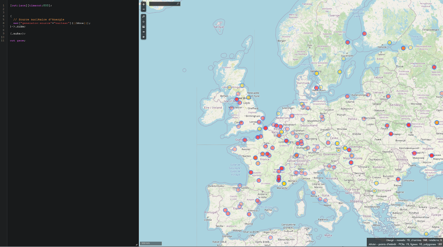
Congratulations, you’ve completed your first Overpass Turbo query! That’s a lot of results, uh?
Second important element, the airport. Given the altitude, we know that an airport is probably close to the position of the plane at the time of the photo. So we go back to our wiki-bible to look for parameters allowing to tag an airport.
Quite quickly, we find the key/value pair aeroway=aerodrome which indicates to be a general element for this type of infrastructure (link). In order to link this new search to the last one, and thus reduce the number of results, we will try to integrate a notion of distance. Thus, we will select all the airports within X kilometers of a nuclear power plant. I advise you to perform different tests in order to visualize the differences in results. There are few elements that allow us to calculate the precise distance. We can say that 20 kilometers is a good distance for a starting point, considering the picture.
Still following the same model, we can add the following block to our query, storing the result in a new variable airport which we will call in the results:
(
  // Aerodrome and airports near to nuclear power plant (<20km)
  nwr(around.nuke:20000)["aeroway"="aerodrome"];
)->.airport;
Which gives the following result :
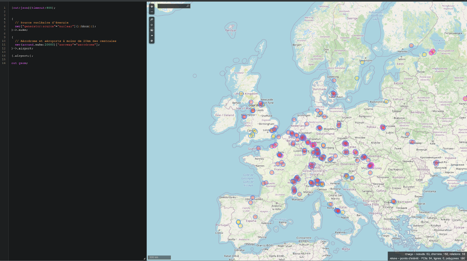
Different results… More clustered… What ? Well yes, by changing the query, we also changed the set of items to display. From the European nuclear power plants, we changed to all the airport infrastructures (including aerodromes!) near power plants. Therefore, if we have 4 results near the same power plant, then all four will be recovered.
From there, two solutions:
- Modify the query to add a 3rd element;
- Or refine the current query by working on the elements already present.
Indeed, in the same way as for the first request, a tag exists on this object and allows to filter on the type of infrastructure, the size. It is the type tag (link). In our case, it seems to be an international object. So we can modify our query accordingly and add the tag in question.
(
  // "International" airports near to nuclear power plant (<20km)
  nwr(around.nuke:20000)["aeroway"="aerodrome"]["aerodrome"="international"];
)->.airport;
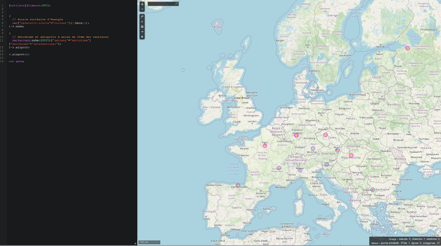
Far less results! From here, we could start looking manually through the 12 airports, but that would still be potentially tedious. Instead, we’ll see if it’s possible to narrow again the list.
To do this, why not add the two additional items identified?
Since roads are rather common infrastructure, the goal could be to first refer to water sources to filter the results. However, we want these water sources to correspond to certain precise criteria:
- They must be close to an airport (necessarily) ;
- They must be very close to a road, which we have to qualify.
To achieve this, we will be able to create a kind of first condition to respect, before carrying out our real research. Thus, we will look for everything that can be related to a water source near our result set. In order to be relatively wide, we can use the key/value natural=water (link). Once again, I advise you to test for distances. On our side, considering the altitude of the plane on the picture, we know that it is quite close to the ground. Without being able to calculate its precise altitude and thus its distance from the airport, we can consider that it will not be 10 kilometers from the point we are looking for… Visually, we can suppose that 3km is still relatively wide. Some tests lead us to see that the results differ little while decreasing the distances. However, below 1km, few results remain. Therefore, 1500 meters seems to be a good starting point.
(
  // Water sources less than 1500m from previously stored airports
  nwr(around.airport:1500)["natural"="water"];
 )->.waterspots;
Then, we can create a second variable to retrieve all the roads very close to the identified water sources. Considering the picture and in order to be wide enough, let’s take a value of 100 meters. Through the wiki, we can identify that the roads are classified under the key highway. The value allows us to classify the different roads according to their size. From the picture, we see a 2-lane road with a median line. It seems to be a major road, but not a highway. The most likely value associated with this type of road is trunk. (link). So :
(
  // Secondary roads less than 100m from all the identified water sources
  nwr(around.waterspots:100)["highway"="trunk"];
)->.road;
Right. Both elements are selected and stored in variables. However, the roads were searched from the water sources, and not the opposite. Indeed, it would have been useless to first search the roads located at 1500 meters from an airport… Because the search would probably have returned results for all airports.
However, we want to filter the airports according to the water sources “matching” our criteria. To do this, nothing deny us from cross-checking the previous results, in order to select only the water sources corresponding to both the distance to an airport and the distance to a major road. We can therefore take our two elements and cross-reference them with each other, for example by searching in our set of water sources for those that are 100m or less away from a major road.
(
  // Linking water sources and roads previously identified
  // Getting matching water sources
  node.waterspots(around.road:100);
  way.waterspots(around.road:100);
  relation.waterspots(around.road:100);
)->.matching_water;
Which gives the following result.
So we gradually built our query to collect:
- Airports close to nuclear power plants in Europe ;
- The set of water sources near these airports, then we processed this data to restrict the number of results (thanks to the road).
Now we just have to cross-reference these two data sets to see which airports match! To do this, we will search in our set of airports, those close to water sources contained in the second set of data.
(
  // Research in the airports dataset those being
  // 1500m or less awway from identified water sources
  node.airport(around.matching_water:1500);
  way.airport(around.matching_water:1500);
  relation.airport(around.matching_water:1500);
)->.matching_airports;
This looks good, uh ?
Final request and results
Putting all of the above together to build a single search query, we get something like this, with some comments :
[out:json][timeout:800];
// gather results
(
  // Nuclear power plants
  nwr["generator:source"="nuclear"]({{bbox}});
)->.nuke;

(
  // Airports less than 20km away from these nuclear sources
  nwr(around.nuke:20000)["aeroway"="aerodrome"]["aerodrome"="international"];
)->.airport;

(
  // Collecting a set of water sources close to airports identified
  nwr(around.airport:1500)["natural"="water"];
 )->.waterspots;

(
  // Getting roads less than 100m away from these water sources
  nwr(around.waterspots:100)["highway"="trunk"];
)->.road;

(
  // Filter the water sources dataset with the previously collected roads
  node.waterspots(around.road:100);
  way.waterspots(around.road:100);
  relation.waterspots(around.road:100);
)->.matching_water;

(
  // Searching in the collected airports those who match all criteria (water sources)
  node.airport(around.matching_water:1500);
  way.airport(around.matching_water:1500);
  relation.airport(around.matching_water:1500);
)->.matching_airports;

(.matching_airports;);

out geom;
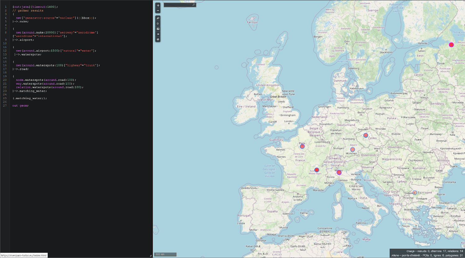
Still focused on Europe, the query can be executed, and after a few minutes of searching (for me) :
So, yes, visually and on a European scale, the same areas are identified. In total, 7 potential zones (which is still much better than our first results!):
- Paris, France
- Lyon, France
- Milan, Italy
- Sofia, Bulgaria
- Munich, Germany
- Prague, Czech Republic
- Saint Petersburg, Russia
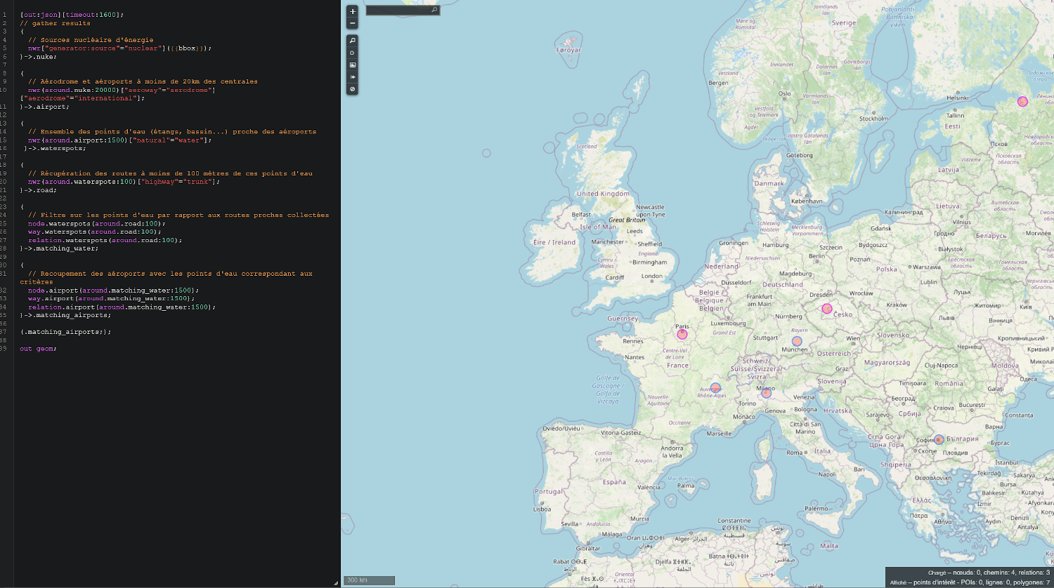
There are several ways to refine the results. For example, the list of 7 airports can be cross-referenced with the list of those served by Easyjet (link), which allows us to eliminate Saint-Petersburg’s airport. We can also rely on the relief present on the photo, allowing us for example to discard airports such as Paris, Munich or Prague, which leaves us a list of 3 areas to check manually:
- Lyon, France
- Milan, Italy
- Sofia, Bulgaria
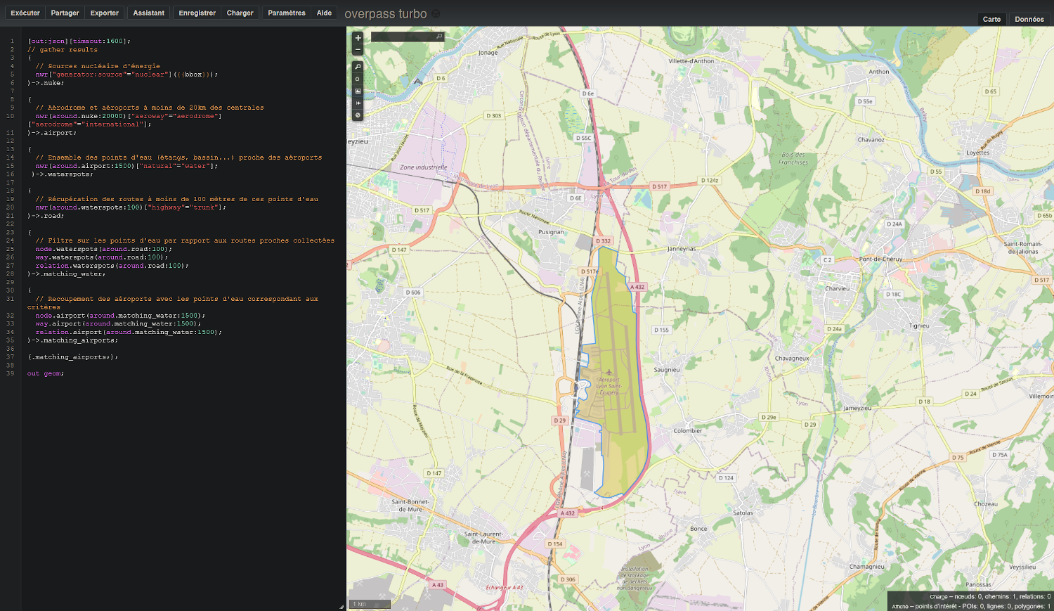
Finally, a new use of Overpass Turbo can be made by targeting one after the other the 3 identified zones. Since the search area is smaller, the query is almost instantaneous. The image below illustrates this with the Lyon airport.
In the same way, we can modify the query to display the different water sources identified before. This is how we can retrieve different water sources identified north of the airport.
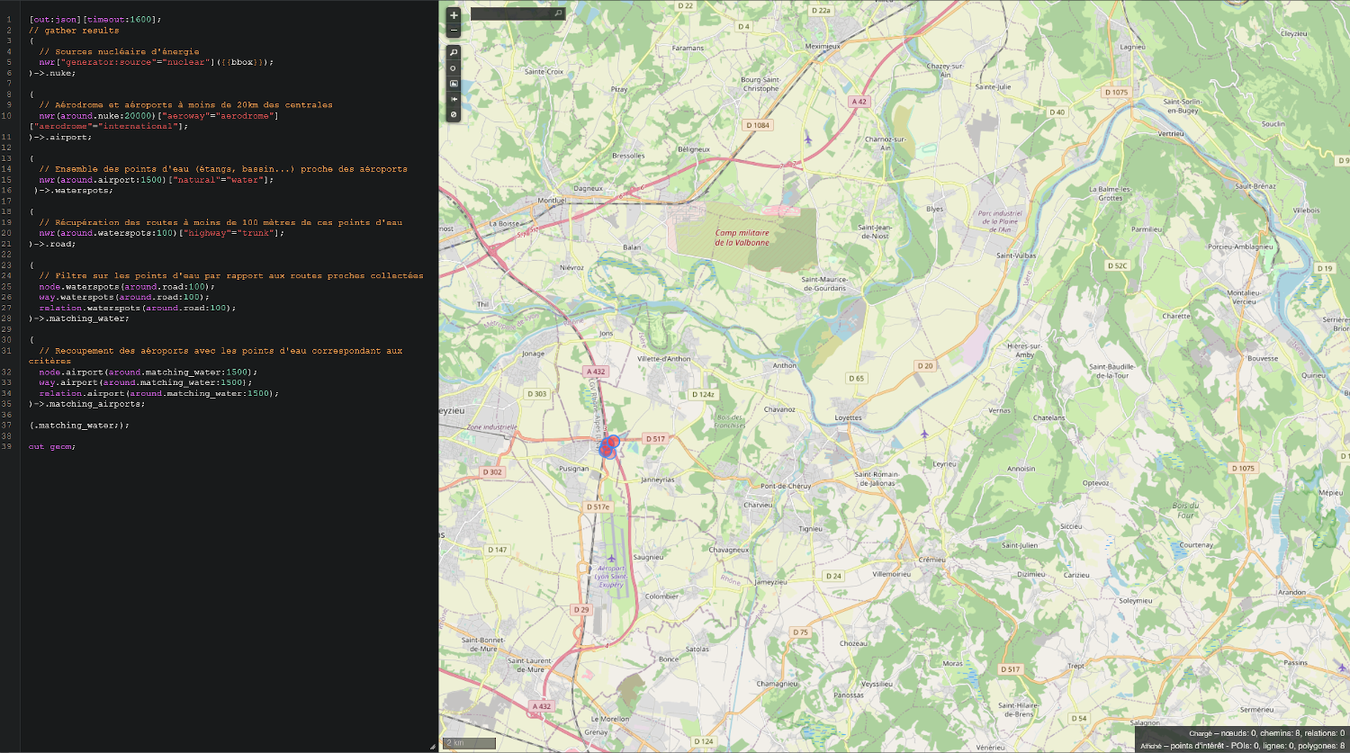
At this point, you have understood, we will be able to carry out the same verification as for the first method using tools such as Google Earth, to validate the geolocation of the place as being the airport of Lyon!
Conclusion
If we go back to the initial statement, which was really just an excuse to talk about Overpass Turbo, then we can say that this person spent his weekend in Lyon! We have thus seen two methods that can be used to help investigate these topics, each with their own advantages, disadvantages and applications!
Indeed, although it is not possible to find the airport of departure using Overpass Turbo, the tool is of course not limited to the aviation field, far from it. If you are interested in this topic, I strongly suggest that you read more about the data collected and available through Open Street Map and the further use of Overpass Turbo, because the tool is really powerful and can be used in many cases.
I didn’t say it in the introduction, but it goes without saying that I am far from being an expert on the tool or more generally on OpenStreetMap related topics, but this was the opportunity to talk about it. In the meantime, I hope that reading this post has taught you some things, or at least entertained you ;-).
Resources and tools
Different resources have been given throughout the article. You will also find them gathered below, as well as a set of other very interesting links related to the subject, if you wish to deepen the use of the tools.
-
Knowledge bases about Overpass Turbo and Open Street Map
-
Other blogposts related to Overpass Turbo
-
Flight Tracking Tools